After 100 SOL in profit and ten months of work, we closed our autonomous trading desk
We started by asking a language model which memecoins to buy and ended with our own data lake, our own LightGBM models and a desk that traded around the clock. This is the whole arc, step by step, including the parts that did not work, and the measurements that told us to stop.
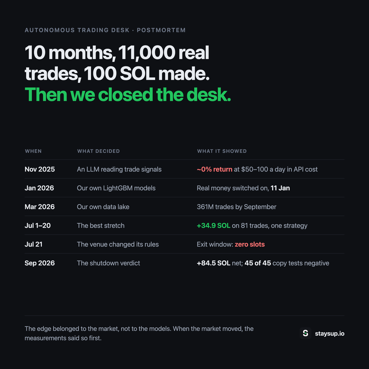
On 11 September we switched off the last strategy that was trading real money. Two weeks later we finished the verification that asked whether that had been the right call, strategy by strategy, against the database and the full trade archive. It was. The desk, which we ran under the name unrekt, made about 100 SOL on the four strategies that worked, and 84.5 SOL net once the four that did not are counted, across nearly 11,000 real trades. At September's price of around $117 a SOL the net is just under $10,000.
This write-up is the story in the order it happened, because the order is the useful part. Each step fixed the problem the previous one exposed, and each fix exposed the next problem. If you are building any system that makes decisions on its own, whether it trades, scores leads or approves payments, most of these steps will look familiar long before the money does.
What the desk traded
The market was pump.fun on Solana. Anyone can launch a token there on a bonding curve, a price formula that rises as people buy. When enough SOL has gone in, about 80 on the curve, the token "graduates" into a normal trading pool. On an ordinary day around 250 tokens graduated. Most of them are worth nearly nothing within an hour, and a small number go up five or twenty times.
That shape, a lot of losers and a few very large winners, is what made it tradeable and what made it dangerous. A strategy there does not need to be right often. It needs to avoid the obvious losers cheaply and be holding when the rare winner runs, and it needs to do both within seconds, because the whole life of an interesting token can be over in fifteen minutes.
Step 1: we asked a language model
The project started in October 2025 as something else entirely, a small web app that read a Solana wallet and showed you how much you had lost on memecoins. Six days later we added a feature where Claude explained your losses to you, and five days after that the obvious question arrived: if the model can explain a bad trade, can it pick a good one?
So we built that. An on-chain scanner found tokens that users of retail trading bots were buying, pulled market data and security checks for each one, and handed the model a prompt with one and five minute candles and the state of our paper portfolio. Claude answered buy or skip, and the bot posted its picks to a Telegram channel. We ran Sonnet, then Haiku to save money, then both side by side. That bot, from the scanner through the Claude step to the points scorer and the hybrid shadow tracker below, is public as unrekt-telbot, a code-only snapshot with every strategy weight set to a neutral 1.
It lasted about two and a half weeks. Our own reality check on 15 November put the return at roughly zero, and the API bill for the Sonnet path was estimated at $50 to $100 a day. The more telling number came from a comparison on the same 741 tokens. The model bought 21.7% of them. A plain points table, the kind of scoring rule you could write on a napkin, bought 66.4%, and caught 3.1 times as many tokens that went on to rise more than 20%. The model was not stupid. It was cautious in a market that pays for being present at the few winners, and nothing in the prompt could tell it which of its hesitations had been expensive, because it never saw an outcome.
That was the first real lesson, and it shaped everything after it. A language model reading a chart has opinions but no label. It cannot learn from the 741 tokens it just watched unless you build the loop that shows it what happened, and once you have built that loop you have built the thing a much smaller, cheaper model needs.
Step 2: rules, then our first model
We replaced the model with the points table on 15 November and, a week later, with the first machine learning model trained on our own outcomes. It had 944 samples and 55.2% accuracy, which is barely better than a coin, and it was still the right move, because now every trade produced a label and every label made the next model better.
On 11 January the first of those models started trading real money. We called it the hybrid: an entry classifier, a tail classifier and crash and upside regressors voting together, buying through a swap aggregator and selling on a fifteen-minute clock. Between January and the end of May it made 3,534 real trades. Its closed trades brought in 11.8 SOL more than they cost. Then 138 trades bought tokens that could never be sold, because the pool drained or the sell kept failing, and those cost 8.45 SOL, so the book finished at about plus 3.4 SOL. Seven in ten SOL of its profit went to exits that did not exist, which is a lesson the curve strategy would teach us again in June.
Over the winter that became a proper pipeline: LightGBM classifiers for whether to enter and whether a token would have a fat tail, regressors for crash risk and upside, 142 features computed from price, liquidity, holder structure and trading flow, and a training script, a backtest and a serving service that all read the same filter definitions from one file. The one-file rule came later than it should have, and the next step is why.
Step 3: the data had to be ours
In March a one-line change to a liquidity filter, made for a sensible reason in the live trading code, quietly changed what went into the training set. At March's SOL price the new rule let in tokens with $6,100 to $7,100 of liquidity, below the old $10,000 floor, so about 28% of the new training rows came from a population the models had never seen. Nothing errored. Models trained with more March data simply did worse on April, in proportion to how much March they had seen. A model trained only on the new data backtested at minus 18.84% per trade, and the one that left March out entirely came in at plus 8.07%. We had seen the same thing once before, in December, after a scanner change.
Twice was enough. On 17 March we started our own collector for pump.fun, reading the chain directly through streaming RPC instead of assembling each token's history from third-party APIs after the fact. Usable data starts on 22 March. By the end the archive held 361 million bonding-curve trades from 20 April to 11 September, in Parquet on cloud storage, with Postgres for the live state and Redis for the hot per-wallet counters.
The collector changed what the models could see, and it also changed the job. We were no longer a trading bot with a model attached. We were a data pipeline that happened to trade, and from then on most of our failures were pipeline failures.
Step 4: real money, and the checks that kept the models honest
The collector's own strategies went to real money at the end of March, nine days after it started, and the hybrid was retired at the end of May. Every strategy from then on ran in two forms at once, a paper version at zero cost and a real one with real fills, so that the gap between them measured our execution rather than our luck.
This is where the comparison checks earned their keep, because nothing they caught would ever have raised an error on its own. The reconciliation that re-scores every production input offline caught the first one. The serving path skipped a step that training performed before its imputer, so about half of all live inputs were scored on training medians instead of zeros. We wrote that one up separately as the train-serve skew. A few weeks later one model rejected every single trade for a different reason: one SQL file divided a quantity by a million and the other did not, so the model saw values a million times smaller than it was trained on and said no to all of them. A retrain lowered the spread of our scores, and a fixed 0.60 threshold that used to pass the top 15% now passed the top 9%, which is the calibration story.
The most expensive lie was in the backtests themselves. Our main sniping model showed a profit factor of 1.69 on a 24-day out-of-sample backtest and was losing money live at 0.94. Part of the gap was tokens that graduate so fast nobody can actually buy them. With those removed, the honest backtest fell to 1.53. A retrain that excluded them lifted AUC from 0.865 to 0.915 and backtested worse, at 1.35. A better score on the metric was a worse strategy.
The same problem went deeper in our curve strategy. On 19 June we proved at the level of individual Solana slots that 32.6% of graduations complete within one block of crossing 80 SOL, too fast for any outside order to get in. Those tokens averaged plus 73% over the next minute, and they were where the model's apparent edge came from. On the tokens we could actually fill, the same rule lost about 7% a trade after costs. Whether a token would be fillable was very predictable, at AUC 0.904, and it did not help, because the fast ones were the profitable ones.
Step 5: the strategies that made it
We redesigned the curve strategy around what could actually be filled, and it became the best stretch the desk ever had. Here is the lifetime result of every Solana strategy that traded real money, from transaction-confirmed fills, where the profit is exactly SOL received minus SOL spent.
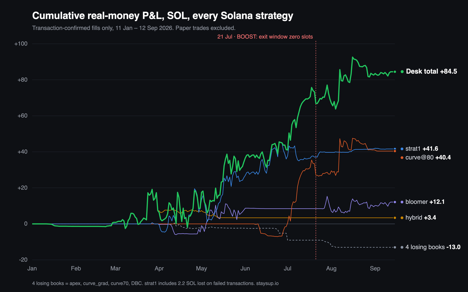
| Strategy | What it did | Real trades | Real SOL |
|---|---|---|---|
| strat1 | Bought freshly graduated tokens on rules, with an ML veto added later | 2,649 | +41.6 |
| curve@80 | Bought on the bonding curve at 80 SOL, just before graduation | 722 | +40.4 |
| bloomer | ML sniper, bought a graduate in its first minute betting on a 5 to 20x | 1,416 | +12.1 |
| hybrid | Four LightGBM models voting, fifteen-minute exits, January to May | 3,534 | +3.4 |
| apex | ML entry and exit at fixed checkpoints after graduation | 2,245 | −2.4 |
| curve_grad | Bought at 40 SOL on the curve, sold before graduation | 197 | −2.8 |
| curve70 | Raced fast graduations from 70 SOL | 147 | −5.2 |
| DBC | The same idea on a different launchpad | 37 | −2.7 |
| Total | winners +97.5, losers −13.0; strat1 is net of 2.2 SOL lost on failed transactions | 10,947 | +84.5 |
The pattern in that table was the most useful single finding of the year, and we only saw it clearly in a profit attribution at the end of July. Everything that won was selection: deciding which token to hold. Everything that lost was speed: racing other bots to the same token in the same second. Speed races were always somebody else's business with better infrastructure. Selection was ours, because it depended on data and models we had built ourselves.
Strat1 was the only book with a statistically solid edge over its whole life, a t-statistic of 2.83 over 2,649 trades. Curve@80 made most of its money in a short window. From 1 to 20 July it made 34.9 SOL on 81 real trades, a pace of about 70 SOL a month from one strategy on a small wallet. For three weeks it looked like a business.
Step 6: the day the venue changed
Around 21 July pump.fun shipped what traders called BOOST mode, a mechanism that spent roughly 17.6 SOL of protocol money buying each newly graduated token. Farmers adapted within a day. Graduations went from about 250 a day to 1,061, many of them tokens months old pushed over the line on purpose, and the typical graduate was down 95% fifteen minutes later.
We tried to trade around it by selling straight into the protocol's buy. In our database simulation it looked excellent. At the slot level it was a phantom. The farmers bundled their sell into the same atomic transaction bundle as the migration and the protocol buy, so the price was already down 6 to 18% by the first swap anyone else could make. The exit window was zero slots. No amount of infrastructure speed fixes that, because to get out in time you would have had to be inside their bundle.
Curve@80 lost 6.5 SOL on 21 July alone, fifteen trades in one day, until our flood guard parked it. What happened next is the fat tail in one picture. Between 21 July and 16 August curve@80 made 14.1 SOL over 185 trades, and 19 SOL of that was a single trade on 7 August that returned 1,857%. Without that one token the stretch lost about 5 SOL. After 16 August it lost 7.1 SOL over 228 trades, and the regime never came back. By September, a typical graduate's price one hour after graduation, measured against its price at five minutes, had fallen from a median of 0.55 to 0.73 in the June and July stretch to 0.01 or 0.02. The median token was simply gone within the hour.
Step 7: keeping it running
An autonomous desk is mostly an operations problem, and it is where the checks we now run for clients were first built. The instructive case is a nightly job that snapshotted our Redis wallet counters to the data lake. One wallet, an industrial trading fleet active in 57,000 tokens, had grown a single value to 3.27 MB, and the CSV reader the job went through refuses any line over 2 MB, so every run aborted while the scheduler still reported the job as running. A cutover test that compared the job's output across a machine migration caught it. The fix raised the limit with the memory budget beside it and kept the biggest wallets, because skipping bad lines would have silently dropped exactly the actors we most wanted to see. The same oversized value also explained a collector memory problem in August, so one diagnosis closed two incidents.
In June our streaming provider stalled for about four and a half hours and then dumped the backlog in huge batches. The collector's own lag figure showed it at once, and the diagnosis ruled out the database and the CPU and found the real shape: the ingest route acknowledged a batch only after processing all of it, so the provider timed out and resent the same batch, and the recovery was what kept the collector behind. It is the same pattern we describe in what breaks at a billion events. Both cases come down to the first rule of our freshness work: measure what a job produces, never only whether it runs.
How autonomous it actually was
Once a model was deployed the system needed nobody. One container ran 24 hours a day, reading the chain, computing features, scoring with the model, sending transactions through two routes at once so the faster one landed, and managing exits. It traded through nights and weekends without a person watching.
Everything around the trading was still ours. A person deployed every release and rolled every model, chose which retrain to promote, changed position sizes, turned gates on and off, diagnosed every incident and made every call to pause or stop. The curve pause on 3 September was a judgement call about the market regime, made by a human reading the numbers. We think that split is the right one for a system like this, and it is the same split we would recommend to anyone putting a model in charge of money: the model decides trades, people decide whether the model should still be deciding.
The graveyard
The table above is only the Solana strategies that reached real money. Our strategy registry lists more than forty lanes in total, and most of them died in paper or in backtests: launchpads on BNB Chain and Base, sniping and copy-trading on Robinhood's chain, market-making on Polymarket, liquidity provision on Meteora, NFT lending. The liquidity-provision engine had a backtest showing 108 SOL a month. Replayed properly against real pool history, zero of fourteen pools were profitable in any of six configurations, because the losses from prices moving against the position ran at about 2.7 times the fees earned. We have written about the same failure in general terms in the strategy life cycle: the backtest is where an idea goes to look good.
The verdict
By early September everything was either paused or losing, and the question was whether to shut down completely or wait for the market. So we verified every strategy that had been active, from confirmed transactions, and went looking for new patterns in the full archive before deciding.
Curve@80 had lost 7.1 SOL over its last 228 real trades, a t-statistic of minus 2.53, the only book that was significantly negative. Its production model, retested out of sample, had an AUC of 0.4985, which is a coin. Strat1 had shrunk to about 0.08 SOL a day. Bloomer was the close call: positive on paper, positive in real money only through 12 take-profit hits that averaged plus 456%, and negative without them.
Then we tested the ideas everyone suggests once. On 361 million curve trades, with wallets ranked only on earlier months and 5% round-trip cost, copying the best-performing wallets lost money in all 45 combinations of wallet count, holding time and month. Waiting for several good wallets to agree lost in 35 of 36. Following creators with a good track record lost in four of five months. Wallet skill on those curves is real and it persists, and it is smaller than the cost of acting on it a few seconds late.
One thing did hold across independent books. When SOL had risen more than 5% over the previous seven days, the next day was bad for every strategy we ran. On the day of the verdict SOL was up 17 to 20% in a week. The one signal we trusted said stay out, so we did.
What we learned
A language model is a poor trader for the same reason it is a good analyst. It reasons about what is in front of it and it never sees how the story ended. The step that made the desk work was not a smarter model. It was owning the data and the labels, so that a small, cheap LightGBM could learn from outcomes the large model never saw.
The failures that cost money in a system like this never raise an error. The March training data, the imputer, the unit mismatch, the unfillable backtest and the stalled snapshot job all looked healthy from the outside. What caught every one of them was a comparison of two numbers that should have been equal: paper against real, production against offline, backtest against live, output today against output yesterday. Those comparisons are the core of what we now build for other teams, and this desk is where we learned which ones matter.
And the edge you find belongs to the market you found it in. We were able to measure, week by week, that there was less of the thing we knew how to trade. The most valuable part of ten months of infrastructure turned out to be the part that let us say so with a t-statistic instead of a feeling.
Built with coding agents
The desk was one person and a lot of AI. Over eleven months the repository reached 2,374 commits from a single author, about 141,000 lines of TypeScript for the collector and trading engine, 123,000 lines of Python for training and research, 17,000 lines of SQL and 752 markdown documents. Most of the code and most of the analysis were written by coding agents working from those documents.
What made that workable was the writing, not the generation. Every investigation ended in a dated document with the query, the sample size and the verdict, and every decision went into a memory the agents read before starting work, so a session in August did not re-run a July experiment or re-open a question we had already closed. The agents were fast, and they were confidently wrong often enough that every number in this article was checked against the database or the archive before it went in. That habit is now the method we publish as receipts-wiki.
What it is not
This is one person's desk on one venue during one unusual year, and 84.5 SOL net over ten months is a modest result. Our cloud infrastructure cost about €6 a day in August and more earlier in the year, when it was closer to $1,000 a month, so the net after costs was smaller still. It is not evidence that you can make money trading memecoins with machine learning, and we would not tell anyone that you can. Only one of eight real-money strategies was statistically significant over its whole life, the best month came from a regime that ended in a day, and a single trade made more than a fifth of the desk's net. The dollar figure uses September's SOL price for convenience; the profit was realized at many different prices.
A few numbers here are estimates or come from our own backtests rather than real fills, and we say so where they appear: the LLM's API cost was an estimate at the time, and the profit factors and per-trade figures in Step 4 are backtest results.
What came next
The ML serving machine was shut down on 14 September and the batch machines after it. The collector and the database are still there for now, as the record, and so is the Parquet archive. The code stays, and the part that ran the first half of this story is open source at unrekt-telbot. We are not planning to restart. If we ever did, the rules for it are already written down: SOL calm for a sustained period, post-graduation prices recovering towards the July levels for a full week, and only the one strategy that was still positive, at a fixed size.
What outlives the desk is the set of checks that caught systems reporting healthy while what they measured had stopped or changed. None of them is specific to memecoins, and they transfer to any pipeline that feeds a model or a decision.
What to do with this on Monday
- If a model makes decisions for you, run a zero-cost paper twin of every decision and chart the gap between the two. It is the only clean measure of execution you will ever get.
- Log the exact inputs the model scored in production, then re-score a sample offline every week. Anything that is not an exact match is a lead.
- For every backtest, ask which of its trades could actually have been executed. Remove the ones that could not and run it again.
- Check the freshness of every scheduled job's output, not whether the job ran.
- Write down the conditions under which you would switch the system off before you switch it on.
Sources: our own trading database and Parquet trade archive (361M curve trades, 20 Apr to 11 Sep 2026), transaction-confirmed real P&L, and the dated investigation documents in the project repository, verified 23 September 2026 and re-checked against the database on 25 September. Code: unrekt-telbot. Related: the strategy life cycle · the threshold that lied · train-serve skew · what breaks at a billion events